Discrete Distributions
Uniform, Binomial distribution concepts, and python code
Utilities Code Functions
This code was run in a Jupyter Notebook
Python Here Import Libraries
1
2
3
4
5
6
7
import numpy as np

from scipy.stats import binom

import matplotlib.pyplot as plt
from matplotlib.animation import FuncAnimation
from IPython.display import HTML
Python Here discrete_uniform_sim()
1
2
3
4
5
6
7
8
9
10
11
12
13
14
15
16
17
18
19
20
21
22
23
24
25
26
27
28
29
30
31
32
33
34
35
36
37
38
39
40
41
42
43
44
45
46
47
48
49
50
51
52
53
54
55
56
def discrete_uniform_sim(frame,
                         low_int=1,
                         high_int = 6,
                         drawn_samples = 1000,
                         ylim=(0,.3),
                        ):
    '''
    Description:
    -----------
        This function simulates an statistical experiement where
        certain number of sample (drawn_samples argument) are drawn
        with replacement from an discrete uniform distribution.


    '''

    #_________________________
    # low_int=1
    # high_int = 6
    # drawn_samples = 1000
    # ylim=(0,.3)

    expected_prob = np.round(1/len(range(low_int,high_int+1)), 4)


    #_________________________
    X = np.random.randint(low=low_int,
                      high=high_int+1,
                      size=drawn_samples)
    x_i, x_count = np.unique(X, return_counts=True)
    x_prob = x_count/drawn_samples

    #-------------------------------------
    expected_mean = np.sum(x_i)/6
    observed_mean = np.sum(x_i*x_count)/1000

    #-------------------------------------
    # VIZ
    # Clear current axes
    plt.cla()

    plt.scatter(x_i, x_prob)
    plt.vlines(x=x_i, ymin=[0]*len(x_i), ymax=x_prob, linestyles='-', label='Observed probability')
    plt.axhline(y=expected_prob, color='r', linestyle='-', label=f"Expected probability {expected_prob}")
    plt.text(x=1, y=ylim[1] - 0.05, s=f"Observed X mean: {observed_mean}\nExpected X mean: {expected_mean}")


    plt.ylim(ylim[0], ylim[1])
    plt.ylabel('Probability')
    plt.xlabel('Discrete sample space of X')

    plt.gcf().set_facecolor('lightgrey')
    plt.gca().set_facecolor('lightgrey')
    plt.title(f"Discrete Uniform Distribution \n Simulation: Drawn {drawn_samples} samples on each experiment")
    plt.legend(title= f"Experiment: {frame+1}", framealpha=0)
Python Here binomial_sim()
1
2
3
4
5
6
7
8
9
10
11
12
13
14
15
16
17
18
19
20
21
22
23
24
25
26
27
28
29
30
31
32
33
34
35
36
37
38
39
40
41
42
43
44
45
46
47
48
49
50
51
52
53
54
55
56
57
58
59
60
61
62
63
64
65
def binomial_sim(frame,
                 n_binomial_trials=40,
                 n_drawn_samples = 1000,
                 ylim = (0,.3),
                ):


    # n_binomial_trials = 100 # in Bernoulli process
    p = np.arange(0.1, .9, 0.01)
    if frame >= len(p):
        p= 0.9
    else:
        p = np.arange(0.1, .9, 0.01)[frame]
    # n_drawn_samples = 10000


    #______________________________________________
    # Simulation
    # drawn_samples = binom.rvs(n=n_binomial_trials,
    #                           p=p,
    #                           size=n_drawn_samples,
    #                           random_state=None,
    #                          )


    drawn_samples = np.random.binomial(n=n_binomial_trials,
                                       p= p,
                                       size=n_drawn_samples)

    sample_space, sample_counts = np.unique(drawn_samples, return_counts=True)
    observed_prob = sample_counts/n_drawn_samples

    #______________________________________________
    # Probability Mass Function (PMF)
    X_binomial =np.arange(1, n_binomial_trials+1)
    expected_prob = binom.pmf(k=X_binomial,
                              n=n_binomial_trials,
                              p=p)

    #_____________________________________________
    # VIZ

    # Clear current axes
    plt.cla()
    plt.scatter(X_binomial, expected_prob, marker='.',c='r', alpha=0.5,#'#ff7f0e'
                label="Expected Probability",
               )
    plt.scatter(sample_space, observed_prob, marker='.', c='#1f77b4')
    plt.vlines(x=sample_space,
               ymin=[0]*len(sample_space),
               ymax=observed_prob, linestyles='-',
               colors='#1f77b4',
               label='Observed probability')

    plt.text(x=1, y=ylim[1] - 0.04,
             s=f"{n_binomial_trials} Bernoulli trials\n{n_drawn_samples} drawn samples")

    plt.gcf().set_facecolor('lightgrey')
    plt.gca().set_facecolor('lightgrey')
    plt.ylim(ylim[0], ylim[1])
    plt.xlabel("Bernoulli trials")
    plt.ylabel("Probability")

    plt.legend(title= f"Success Probability p: {p:.2f}", framealpha=0)
    plt.title(f"Binomial Distribution \n Simulation: Drawn {n_drawn_samples} samples on each success probability $p$")
Discrete Uniform Distribution
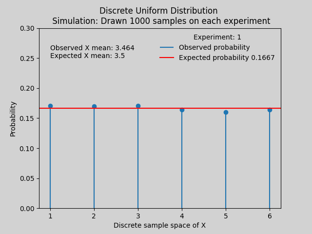
A random variable X has a discrete uniform distribution if each of the n element in its sample space (S), $x_1, x_2, x_3, …, x_n $ has equal probability. Then the probability of each element is given by $f(x_i) = \frac{1}{n} $.
Additionally,
- the expected mean is $\mu = \frac{1}{n} \sum_{i=1}^{n} x_i$ and
- variance $\sigma^2 = \frac{1}{n} \sum_{i=1}^{n} (x_i - u)$
Python VIZ Uniform Simulation Here
1
2
3
4
5
6
7
8
9
%matplotlib notebook
ani = FuncAnimation(fig=plt.gcf(),
                    func=discrete_uniform_sim,
                    frames=range(50),
                    interval=200, # ms
                   )
plt.gcf().set_facecolor('lightgrey')
# ani.save('discrete_uniform_distribution.gif', writer='pillow', fps=5)
HTML(ani.to_jshtml())
Note:
np.random.randint()generates random values based on an uniform distribution.
Binomial Distribution
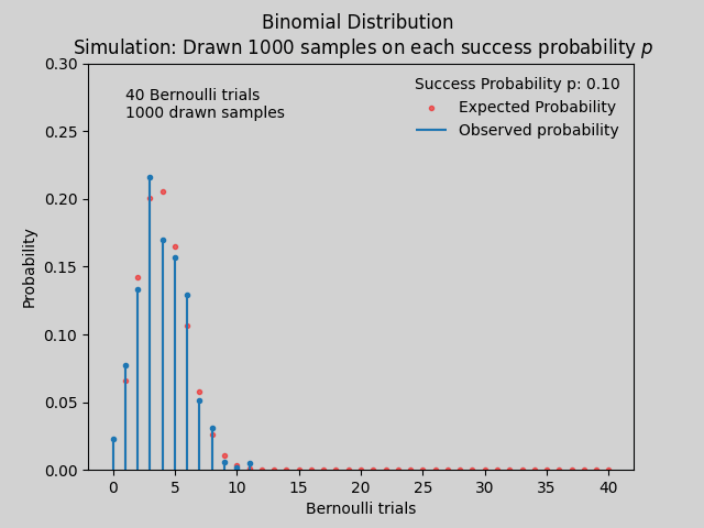
- Binomial distribution is a discrete probability distribution that models the number of successes in a fixed number of independent Bernoulli trials.
- The Bernoulli trial is a statistical experiment that can produce two outcomes: success (with probability $p$) or failure (with probability $1-p$). For example, tossing a coi.n
- Bernoulli Process:
- Process consist in the execution of n Bernoulli trials.
- Each trials will be a success or a failure.
- The probability of sucess $p$, remains constant from trial to trial.
- The repeated trial are independent. The number of success in $n$ Bernoulli trials (Bernoulli process) will be our binomial random variable. The probability distribution of this discrete random variable is called Binomial Distribution.
Example: Setting 3 Bernoulli trials, determine the sample space of the binomial random variable X {0: failure, 1: sucess}:
| Bernoulli Trials | X |
|---|---|
| 0 0 0 | 0 |
| 0 1 0 | 1 |
| 0 0 1 | 1 |
| 1 0 0 | 1 |
| 0 1 1 | 2 |
| 1 0 1 | 2 |
| 1 1 0 | 2 |
| 1 1 1 | 3 |
Each row represents a possible combination result from a Bernoulli process. Therefore, the sample space of X will be {0, 1, 2, 3}
Example: If we said that the probability of success is $p = 0.25$ we could calculate the the probability of obtaining one of those rows as results. P(0 1 0) = P(0)P(1)P(0) = (1-0.25)(0.25)(1-0.25) = $\frac{9}{64}$. Doing this calculation and agregating for each element of the sample space of X we get:
| x | 0 | 1 | 2 | 3 |
|---|---|---|---|---|
| f(x) | $\frac{27}{64}$ | $\frac{27}{64}$ | $\frac{9}{64}$ | $\frac{9}{1}$ |
Python VIZ Binomial Simulation Here
1
2
3
4
5
6
7
8
9
%matplotlib notebook
ani = FuncAnimation(fig=plt.gcf(),
                    func=binomial_sim,
                    frames=range(120),
                    interval=200, # ms
                   )
plt.gcf().set_facecolor('lightgrey')
# ani.save('binomial_distribution.gif', writer='pillow', fps=5)
HTML(ani.to_jshtml())
As the number of Bernoulli trials (n) in a binomial distribution increases, while keeping the probability of success (p) constant, the shape of the Probability Mass Function (PMF) of the binomial distribution begins to resemble more closely the bell shape of a normal distribution. Here, I only show 40 Bernoulli trials. If I were to add, let’s say, 100 trials, it would look even more like a bell shape.
Note:
np.random.binomial()andscipy.stats.binom.rvs()generate random values based on a binomial distribution.
Solving Problem with Binomial Distribution
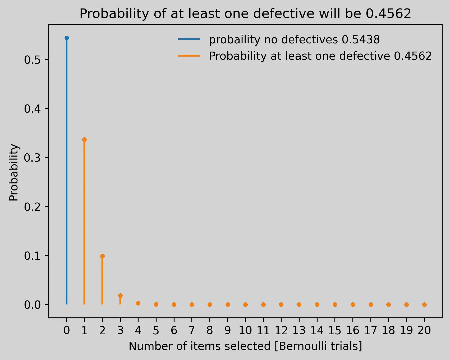
The production line has a defective rate of 3%. What is the probability of finding at least one defective item within 20 randomly selected products?
Code Here
1
2
3
4
5
6
7
8
9
10
11
12
13
14
15
16
17
18
19
20
21
22
23
24
25
26
27
28
29
30
31
32
33
34
35
36
37
38
39
40
41
42
43
44
45
46
47
48
49
50
51
52
53
54
%matplotlib inline
#_______________________________________________
# PARAMETERS
k = 20                # Number of bernoulli trials (20 products in this case)
x = np.arange(0,k+1)  # generating success count range from 0 to 20.
defective_prob = 0.03 # success probability is related to what we want to find.

#_______________________________________________
# USING PMF FUNCTION FROM scipy.stats.binom.pmf()
# Probability Mass function (PMF) to generate the probabilities of each success count.
probabilities = binom.pmf(k=x,  # array of success count to calculate probabilities.
                          n=k, # total of bernoulli trials
                          p=defective_prob,
                          loc=0)

# variable probability is an array with 21 element which indexes represent the number of success.

#_______________________________________________
# INTERPRATATION
# at least one defective means 1 or more success in the 20 randomly selected product.
at_least_one_defct_proba = probabilities[1:].sum()


# 0 success which means 0 defective probability
zero_defct_proba = probabilities[0]

#_______________________________________________
# VIZ
plt.scatter(x, probabilities, marker='.', c='#1f77b4')
plt.vlines(x=x ,
           ymin=[0]*len(x),
           ymax=probabilities,
           linestyles='-',
           colors='#1f77b4',
           label=f'probaility no defectives {zero_defct_proba:.4f}',
          )

plt.scatter(x[1:], probabilities[1:], marker='.', c='#ff7f0e')
plt.vlines(x=x[1:] ,
           ymin=[0]*len(x[1:]),
           ymax=probabilities[1:],
           linestyles='-',
           colors='#ff7f0e',
           label=f'Probability at least one defective {at_least_one_defct_proba.sum():.4f}',
          )
plt.xticks(ticks=x, labels=[str(label) for label in x])
plt.xlabel("Number of items selected [Bernoulli trials]")
plt.ylabel("Probability")
plt.title(f"Probability of at least one defective will be {at_least_one_defct_proba.sum():.4f}")
plt.legend()
# plt.savefig('PMF_binomial_distribution.jpg',
#             dpi=300, # useful for papers publications.
#             bbox_inches='tight')
plt.show()
Note:
scipy.stats.binom.pmf()return Probability Mass Function (PMF) for binomial distributions.
Concepts
Probability Mass Function (PMF)
- PMF directly provides the probability of each element in the sample space of the discrete random variable.
- The set of ordered pairs $(x, f(x))$ is a PMF a.k.a. probability function, probability distribution (Walpole et al., 2007)>chapter3.
- PMF satisfies the following properties:
- $f(x) \geq 0$
- $\sum_{x}f(x) = 1$
- $P(X = x) = f(x)$
References
- Walpole, R. E., Myers, R. H., Myers, S. L., & Ye, K. (2007). Probability and statistics for engineers and scientists. New York: Macmillan.


