Continuous Distributions
Normal distribution with python code
Utilities Code Functions
This code was run in a Jupyter Notebook
Python Here Import Libraries
1
2
3
import numpy as np
import matplotlib.pyplot as plt
from scipy.stats import norm
Python Here norm_sim()
1
2
3
4
5
6
7
8
9
10
11
12
13
14
15
16
17
18
19
20
21
22
23
24
25
26
27
28
29
30
31
32
33
34
35
36
37
38
39
40
41
42
43
44
45
46
47
48
49
50
51
52
53
54
55
56
57
58
59
60
61
62
63
64
65
66
67
68
69
70
def norm_sim(frame,
             mu=0,
             sd=1,
             count_sampes=10000,
            ):

    """
    Parameters:
    ------------
        mu: center location of the normal distribution
        sd: standard deviation
    """

    #_______________________________________________
    # GENERATING RANDOM VALUES FROM NORMAL DISTRIBUTION
    rng = np.random.default_rng(seed=0) # adding a seed.
    random_numbers = rng.normal(loc=mu,
                                scale=sd,
                                size=int(((count_sampes)/50)*(frame+1)),
                               )

    #__________________________________________________
    # CREATING A NORMAL DISTRIBUTION PDF WILL HELP TO
    #   VIZUALLY VERIFY IF THESE VALUES COME FROM A NOORMAL DISTRIBUTION
    x = np.linspace(min(random_numbers), max(random_numbers))
    pdf = norm.pdf(x=x,      # list-like set of x value to calculate the PDF
                   loc=mu,   # location means where is the center, it's the mean.
                   scale=sd, # here scale refers to standard deviation
                  )


    #_____________________________________________
    # VIZ

    # Clear current axes
    plt.cla()  # Clear current axes
    plt.clf()  # Clear the current figure


    # plt.figure(figsize=(12,8)) # this should be outsite of FuncAnimation()
    ax = plt.subplot(121)  # Create subplot
    plt.scatter(np.arange(len(random_numbers)), random_numbers, c='#1f77b4', alpha=0.1,)
    plt.xlabel("Sample count")
    plt.title(rf"Generation of random values from $n(x, \mu={mu},\sigma={sd})$")
    plt.gca().set_facecolor('lightgrey')
    plt.ylim(-4,4)
    plt.xlim(0, count_sampes)

    ax = plt.subplot(122)  # Create subplot
    plt.hist(random_numbers,
             orientation='horizontal',
             bins=100,
             cumulative=False,
             density=True,
             color='#1f77b4',
            )

    plt.plot(pdf, x, 'r-', lw=2, alpha=.5, label="PDF")
    plt.title("Histogram of the generated random values")

    plt.ylim(-4,4)
    plt.xlim(0, .5)
    plt.xlabel("density")
    plt.legend(framealpha=0)
    plt.gcf().set_facecolor('lightgrey')
    plt.gca().set_facecolor('lightgrey')

    plt.suptitle("Normal Distribution simulation")
    plt.tight_layout()
Normal Distribution
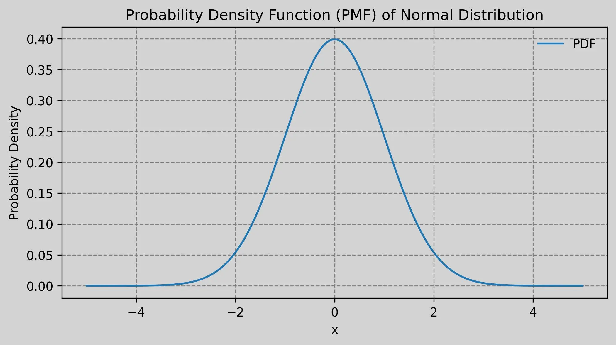
The normal distribution, also known as the Gaussian distribution, is a continuous probability distribution where values are symmetrically distributed mostly around the mean, forming a bell shape. It is characterized by two parameters: the mean and the standard deviation, which determine the distribution’s appearance. A continuous random variable that exhibits this bell-shaped behavior is called a normal random variable.
Probability Density Function:
\[f(x) = \frac{1}{\sigma\sqrt{2\pi}} e^{ -\frac{1}{2} \left(\frac{x - \mu}{\sigma}\right)^2 }\]Python VIZ Here
1
2
3
4
5
6
7
8
9
10
11
12
13
14
15
16
17
18
19
20
21
22
23
24
25
26
27
28
29
30
31
#_______________________________________________
# PARAMETERS
# Define the range
x = np.linspace(-5, 5, 1000) # array of values for "x" in f(x)
mu = 0  # mean
sd = 1  # standard deviation (sigma)

#_______________________________________________
# PROBABILITY DENSITY FUNCTION TO GENERATE BELL SHAPE
pdf = norm.pdf(x=x,      # list-like set of x value to calculate the PDF
               loc=mu,   # location means where is the center, it's the mean.
               scale=sd, # here scale refers to standard deviation
              )

#_______________________________________________
# VIZ
plt.figure(figsize=(8, 4),
           facecolor='lightgrey'
          )
plt.plot(x, pdf, label='PDF', color='#1f77b4')
plt.title('Probability Density Function (PMF) of Normal Distribution')
plt.xlabel('x')
plt.ylabel('Probability Density')
plt.legend(framealpha=0 # transparent backround label.
          )
plt.gca().set_facecolor('lightgrey')
plt.grid(color='gray', linestyle="--", zorder=0 )
# plt.savefig('PDF_nrormal_distribution.jpg',
#             dpi=300, # useful for papers publications.
#             bbox_inches='tight')
plt.show()
Analytical Thought Process
- Consider the bell-shaped curve as a potential model to describe observed data distribution.
- Apply statistical techniques to test if the observed data fit the bell-shaped curve.
- If there is a good fit, we may conclude we have a normal random variable, which allows for parametric analysis.
Notes:
scipy.stats.norm.pdf()return Probability Density Function (PDF) for normal distributions.
Python VIZ Here
1
2
3
4
5
6
7
8
9
10
11
%matplotlib notebook

fig = plt.figure(figsize=(12,8))
ani = FuncAnimation(fig,
                    func=norm_sim,
                    frames=range(50),
                    interval=200, # ms
                   )
plt.gcf().set_facecolor('lightgrey')
# ani.save('normal_distribution_simulation.gif', writer='pillow', fps=5)
HTML(ani.to_jshtml())
Notes:
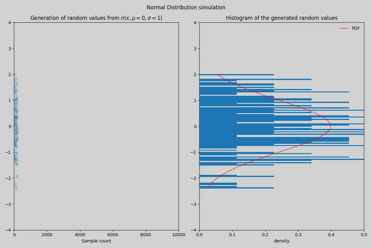
np.random.normal()generate random values from a normal distributions.
Concepts
Probability Density Function
- The probability of a continuous random variable X assuming any exact value is 0. However, the value of the PDF at a particular point can indeed be greater than 0. This means that the PDF value does not equate to a probability but rather indicates the relative likelihood of X being near that value. To obtain probability from the PDF, we need to calculate the area under the curve between two points of X.
References
- Walpole, R. E., Myers, R. H., Myers, S. L., & Ye, K. (2007). Probability and statistics for engineers and scientists. New York: Macmillan.
This post is licensed under CC BY 4.0 by the author.


